Previous
Gradient Descent
Contents
Table of Contents
Next
Clustering

Chapter 10

Ensemble Learning

10.1. Overview

This chapter introduces a very useful machine learning technique, ensemble learning, which can turn multiple models into a more powerful model. We will first study the basics of ensemble learning, including its definition, basic questions, major categories of algorithms, history, and challenges to figure out how it works, why it works, and what to use to make it work better. Next, three major categories of ensemble learning algorithms, i.e., bagging, boosting, and stacking, will be explained. The basic ideas and representative algorithms of these three categories of ensemble learning will be discussed with strict mathematical formulations and pseudo-code for guiding their applications.

10.2. Basics of Ensemble Learning

10.2.1. Definition

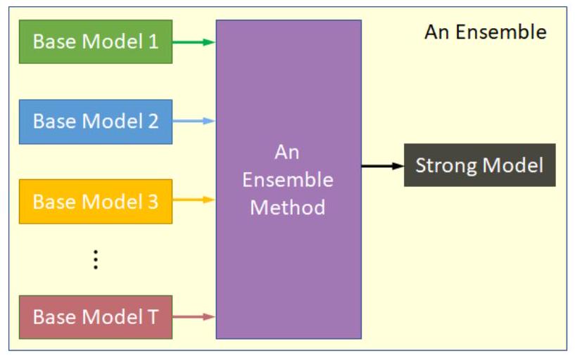
Ensemble learning is a machine learning technique in which multiple models are strategically generated and combined to obtain an ensemble as a model with better performance than that of individual constituent models. As shown in Fig. 10.1, these constituent models, which are called base models or weak models, can be generated with a basic machine learning algorithm such as linear model, SVM, decision tree, KNN, and NN, or their combinations. The former is called homogeneous, while the latter is heterogeneous. Currently, homogeneous base learners are more frequently used. Among them, CART decision tree and neural network are the most frequently used algorithms for constructing homogeneous base learners.
Figure 10.1: Conceptual illustration of ensemble learning
Essentially, the goal of ensemble learning is to create a model whose prediction bias and variance are comparable to or better than what can be obtained with a single base model. There are different strategies for creating an ensemble of base models, leading to different categories of ensemble learning algorithms. The idea behind ensemble learning can be described as "Union is Strength" or "Many hands provide great strength." Therefore, ensemble learning is also viewed as
an optimization method that generates a strong learner from several weak learners.
The process of ensemble learning may contain extensive use of samplings, training of different models, selection and weighing of different models, and most importantly, combining the results from different base models to generate the final prediction for the whole ensemble. Common combination rules for regression tasks are primarily algebraic combiners, e.g., mean, sum, weighted sum, product, maximum, and median, and for classification tasks are primarily voting-based methods, e.g., majority vote and plurality voting. The simplest ensemble learning can be implemented by combining the predictions made by several base learners that are trained on the same training set, though the current mainstream ensemble learning does not refer to such a primitive way of ensembling.
In the remainder of this section, let us first take a quick look at some examples to understand "whether", "when" and "why" ensemble learning works. Then, the common categories of ensemble learning algorithms as well as concepts such as combination rules will be introduced. Finally, we will provide more details regarding the performance of ensemble learning by discussing bias and variance in association with different categories of methods.

10.2.2. Basic Questions

First, let us work on "whether" and "when" ensemble learning can generate a model that is better than the base models used for creating this model. Considering that we have not learned any ensemble learning strategies, let us start with a very simple example in which three cases use a basic combination strategy, plurality voting, as illustrated in Fig. 10.2. Plurality voting here means selecting the label that receives the highest number of votes. As shown, in each case, the predictions of the three base models are combined in a simple way using plurality voting for a binary classification task.
A first look at the three examples can reveal one fact: a group of models, or the ensemble (model) represented by this group of models, does not necessarily exhibit a performance that is better than that of the base models. In fact, the three cases showed discrepant outcomes: (a) the ensemble improves the performance, (a) the ensemble does not take any effect, and (c) the ensemble reduces the performance. Thus, the result provides insights into the "whether" question: ensemble learning can generate better performance in some cases.
Sample 1 Sample 2 Sample 3
Model 1 - + +
Model 2 + - +
Model 3 + + -
Ensemble + + +
True + + +
Sample 1 Sample 2 Sample 3 Model 1 - + + Model 2 + - + Model 3 + + - Ensemble + + + True + + +| | Sample 1 | Sample 2 | Sample 3 | | :---: | :---: | :---: | :---: | | Model 1 | - | + | + | | Model 2 | + | - | + | | Model 3 | + | + | - | | Ensemble | + | + | + | | True | + | + | + |
(a) Ensemble improves performance
Sample 1 Sample 2 Sample 3
Model 1 - + +
Model 2 - + +
Model 3 - + +
Ensemble - + +
True - + +
Sample 1 Sample 2 Sample 3 Model 1 - + + Model 2 - + + Model 3 - + + Ensemble - + + True - + +| | Sample 1 | Sample 2 | Sample 3 | | :---: | :---: | :---: | :---: | | Model 1 | - | + | + | | Model 2 | - | + | + | | Model 3 | - | + | + | | Ensemble | - | + | + | | True | - | + | + |
(b) Ensemble takes no effect
Sample 1 Sample 2 Sample 3
Model 1 - - +
Model 2 + - -
Model 3 - + -
Ensemble - - -
True + + +
Sample 1 Sample 2 Sample 3 Model 1 - - + Model 2 + - - Model 3 - + - Ensemble - - - True + + +| | Sample 1 | Sample 2 | Sample 3 | | :---: | :---: | :---: | :---: | | Model 1 | - | - | + | | Model 2 | + | - | - | | Model 3 | - | + | - | | Ensemble | - | - | - | | True | + | + | + |
(c) Ensemble reduces performance
Figure 10.2: Examples of ensemble learning
A closer look at the example can provide more hints for the answers to the "why" and when" questions. Case 1 shows "why" ensemble learning can improve the performance of base models: different models can complement each other. By contrast, Case 2 and Case 3 show "when" ensemble learning may not work. In Case 2, all the models provide the same predictions, and thus predictions made by combining them make no improvements. That indicates that the base models need to be different from each other to some extent so that the ensemble can be meaningful. Case 3 implies that base models need to be good to some extent to ensure that the ensemble will lead to positive instead of negative changes in the performance. One extreme case is that an ensemble of models that provide random predictions cannot generate a better model, no matter how many such models are used or how these models are combined. In summary, the base models need to be good and diverse to some extent to ensure the ensemble can be effective.
Next, let us check a simple example that can help us understand why ensemble learning can work without touching complicated theories. As shown in Fig. 10.3, a binary classification problem can be solved with simple machine learning algorithms such as a linear model and an SVM. Such models can virtually generate a linear hyperplane, i.e., a straight line in the above 2D example, to separate the data into two groups. This can work well in linear problems.
However, this is not the case when a problem is nonlinear: an optimal boundary to separate the two categories is obviously not a straight line. As illustrated, three base models are generated using linear base models like SVM. Each of these base models can generate a straight line to separate the data. In this case, we can combine the predictions of these three models, i.e., the three straight lines, in some way to generate a nonlinear boundary for separating the two categories of data points. In this way, we obtain an ensemble that can better address this nonlinear binary classification problem
Figure 10.3: Illustration of ensemble learning process
by unifying the strengths of the three base models. This provides a very simple but intuitive demonstration to show why ensemble learning can work.

10.2.3. Categories of Ensemble Learning Methods

There are three common categories of ensemble (learning) methods: bagging (e.g., basic bagging), boosting (e.g., AdaBoost, Gradient Boosting), and stacking [98]. Because ensemble learning involves a process of making decisions with many decision-makers, these three categories are analogous to three concepts in politics. That is, bagging, boosting, and stacking are analogous to pluralist democracy, elitist democracy, and hierarchy, respectively.
As shown in Fig. 10.4, the idea behind bagging is "pluralism". For this purpose, many models can be trained parallelly (or simultaneously and independently), and these models generate the final prediction as the decision of the ensemble via some types of voting or averaging methods. We know that such a pluralistic democracy mechanism will help reduce the differences between prediction results as we attempt to find the average or majority. Therefore, bagging helps reduce the variance of the prediction. Bagging uses bootstrap sampling (sampling with displacement: placing drawn samples back for future sampling) to ensure diversity between base models.
Figure 10.4: Categories of ensemble learning algorithms
By contrast, the idea behind boosting is "elitism". For this purpose, the models are generated in a serial or sequential way so that late-generated models can improve the prediction accuracy based on the performance of early models in the series or sequence. As a result, we can generate "elites" or models with better performance. Such models are generated by
focusing more on samples that are previously incorrectly predicted and are assigned greater weights in the combination of predictions. This effort at the search for better models essentially helps improve the bias of the prediction.
The third category of ensemble learning algorithms attempts to generate a better model from a group of base models by exploring better combination approaches. Intuitively, this can be done by simply combining the predictions of base models with simple combination rules. However, as can be seen, both bagging and stacking involve the use of such basic combination rules. Thus, simple combination via a basic combination rule is not frequently studied. In some literature, basic combination via a simple combination rule is introduced as a more basic category underneath or before bagging, boosting, and bagging, or even merely as combination rules instead of a distinct category of ensemble learning algorithms. In fact, stacking as a more advanced combination approach is predominant in this third category of ensemble learning algorithms. This is why stacking is viewed as the third category in many places. Stacking differs from simple combination rules in that a machine learning algorithm is adopted to learn how to combine the results generated by the base learners for the final prediction. Therefore, this type of algorithm has a two-layer structure: base models and a combination model (or called combiner or final estimator).

10.2.4. Essence of Ensemble Learning

As mentioned above, bias and variance, which measure the performance of predictions, are important concepts that help us understand the goals and outcomes of ensemble learning methods [99]. Here, let us provide more information about them so that we can get a better understanding of the different categories of algorithms. Fig. 10.5 illustrates how bias and variance can reflect on the prediction results. In the context of ensemble learning, bias describes the differences between the prediction and the true label, while variance measures the difference between models, i.e., base models. A high bias implies that the model is not accurate, while a high variance may indicate overfitting.
Figure 10.5: Different conditions of bias and variance
The relationship between bias and variance in machine learning is interesting and essentially related to the understanding and implementation of ensemble learning. There is a tradeoff between these two parameters. In a simple way, as shown in Fig. 10.6, a more complicated model can provide better predictions in theory. Accordingly, the bias will be low. Due to the same reason, the model will turn out to be more sensitive to (new) data, and thus cause a high variance, which may lead to poor performance in the testing data.
A good model should strike a balance between bias and variance. Ensemble learning is such an approach for striking the balance. Usually, bagging starts from the left of the optimum, so it usually has a high requirement on the bias. That is, the performance of the base models is expected to be relatively high. Boosting starts from the right of the optimum, so the base models can have relatively low performance, but the diversity between models needs to be relatively high to ensure a good ensemble learning outcome.
Therefore, in order to reduce the total error using ensemble learning, we will need to find ways to (1) reduce bias (performance of the base models), (2) improve variance (diversity of the base models), and (3) find better combination methods to generate a lower error with given bias and variance of the base models. Item 1 is associated with the selection and implementation of base models, so it is not in the context of ensemble learning. As for Item 2, disturbance
Figure 10.6: Variation of bias and variance with model complexity
to instances, attributes, output, and model parameters (e.g., hyperparameters) can enhance diversity. For example, the bootstrap sampling in bagging is a disturbance to instances, and the random selection of attributes in a random forest is a disturbance to attributes. Item 3 has a good example: stacking. The above understanding can be used as potential tricks for improving the performance of ensemble learning in more advanced applications of this technique.

10.2.5. History and Challenge

To obtain a complete understanding of ensemble learning, let us take a look at the history and challenges of ensemble learning. The concept of ensemble learning was first proposed by Dasarathy (1979) [100], who used linear models and KNN to form composite systems for classification. In the same year, a sample method that was later widely adopted in ensemble learning, i.e., bootstrap, was proposed by Efron [101]. Kearns (1988) and Valiant (1989) proposed the concept of weak learning, which triggered discussions on whether a group of weak learners can create a strong learner [102, 103]. Schapire (1990) provided a positive answer to the question and presented boosting [104]. A few years later, Schapire and Freund proposed the AdaBoost algorithm for boosting, which was awarded the famous Gödel Prize in the area of theoretical computer science [105]. Hensen (1990) proved the variance reduction characteristic of ensemble learning, which can be used to improve the performance of neural networks [106]. The concept of stacking was first proposed by Wolpert (1992), which could help achieve performance better than that of individual learners [107].
In 1995, random forest as one of the most well-known ensemble learning (bagging) algorithms was proposed. In 1996, Breiman proposed bagging based on the understanding of the influence of disturbance on the structure of instances, which affects the variance and, consequently, the learning outcome [108]. Kalal (2010) showed the performance improvements of binary classifiers attributed to the treatment of the structure of instances, and bootstrapping was used for this purpose [109]. Deng et al. (2012) suggested scalable stacking and learning for building deep architectures [110]. A more recent breakthrough is the release of XGBoost by Chen and Guestrin in 2016 [111], which was developed based on many existing techniques, such as GBDT (Gradient Boost and Decision Tree), regularization, shrinkage (change in learning rate), column subsampling, and parallelization, and was later widely adopted due to its outstanding performance.
Despite the advances, ensemble learning also faces challenges for further development. One major challenge is the time-demanding and computationally expensive process of training multiple (base) models. In addition to this general challenge, different categories of ensemble learning algorithms also have their own issues. As for bagging, the use of bootstrapping is based on many statistical hypotheses, whose validity affects the sampling accuracy and learning outcome. Boosting can be excessively sensitive to noise in labels, i.e., outlier, as it attempts to give incorrect predictions higher weights in the sequential learning process. Stacking is challenged by the determination of hyperparameters.
Ensemble learning can be considered in the following application scenarios:
  • Selection of algorithm. It could be tricky to select an appropriate machine learning algorithm. Ensemble learning can help circumvent this issue as it can include many different types of algorithms. This helps save the effort of finding the best algorithm for the given data and reduces the risk of selecting an inappropriate model.
  • Too much or little data. When a dataset is too large, we can split the dataset into subsets directly to train different sub-models; when the dataset is too small, bootstrap provides a good sampling tool for generating subsets from a small dataset.
  • Complex problems. Many problems cannot be well addressed by a single machine learning model, such as classifi-
    cation problems with very complex, irregular (highly nonlinear) boundaries between different categories. Ensemble learning can address such problems by integrating the predictions of different sub-models.
  • Data fusion. Many applications involve data from different sources. Such data from different sources can require the use of different models/algorithms for treatment. Ensemble learning can meet this need.
  • Confidence estimate. Ensemble learning, by nature, can provide an estimate of confidence by investigating how decisions are made by different sub-models. For example, the situation in which most sub-models make the same prediction implies a high level of confidence. Though a high confidence level does not guarantee a good prediction, it was found that with proper training, a high confidence level usually implies a correct prediction and vice versa.

10.3. Bagging

Bagging attempts to obtain an ensemble learning model with high generalization. For this goal, the base learners need to be as mutually independent as possible. A straightforward way to ensure such independence is to divide the training data into mutually exclusive subsets. However, this may lead to insufficient samples for each subset, making the distributions of variables in the subsets different from those in the training data, especially when data is limited. An effective way to address this issue is bootstrap sampling. That is also where the name "Bagging" comes: Bootstrap AggreGating.
Bagging is a very straightforward category of ensemble learning algorithms - it does not necessarily involve complicated theories to guide its implementation. As a result, no equations or deductions are needed in this section. Instead, in the following, extra information including bootstrap sampling, base learners, combination, and pseudo-code will be offered for the basic version of bagging, or called bagging meta-estimator. Then, a popular and more advanced bagging algorithm, i.e., random forest, will be introduced. In particular, the changes that need to be made to move from basic bagging to random forest will be explained.

10.3.1. Basic Bagging

When bootstrap is used, we select a certain number of samples (between 1 and the total number of samples) to form a subset each time and put the selected samples back before generating the next subset. Though it appears to be very simple, this sampling method is very effective in striking a balance between achieving the independence of subsets and letting each subset represent the total dataset in terms of variable distributions (hints: each attribute represents a variable).
In some literature, each subset is also called a bootstrap sample. Therefore, a bootstrap sample is a small sample that is "bootstrapped" from a large sample, which corresponds to the original (training) dataset. Bootstrapping can be interpreted as a type of resampling where many subsets (or sub datasets) of the same size are repeatedly generated, with replacement, from a single original dataset (dataset).
One thing that needs to be mentioned is the Out-Of-Bag (OOB) data. OOB refers to the samples that have not been selected after all the needed subsets are generated. We can use a very simple example to understand it. Let us assume we have a dataset consisting of I I III samples. We select 1 sample from it each time for I I III times to create I I III subsets. Then we know that the percentage of samples that will not be selected in this process is ( 1 1 I ) I 1 1 I I (1-(1)/(I))^(I)\left(1-\frac{1}{I}\right)^{I}(11I)I. The probability as I I III approaches infinite is lim I ( 1 1 I ) I = 1 e 0.368 lim I 1 1 I I = 1 e 0.368 lim_(I rarr oo)(1-(1)/(I))^(I)=(1)/(e)~~0.368\lim _{I \rightarrow \infty}\left(1-\frac{1}{I}\right)^{I}=\frac{1}{e} \approx 0.368limI(11I)I=1e0.368. The real probability varies as the size of the subset and I I III change, but OOB exists due to such a probability. OOB is useful in several ways. First, it can be utilized to replace a separate testing dataset for error estimate, which is called OOB estimate, which is an unbiased estimate compared with the test set. In addition, if decision trees are used as the base models, OOB can be employed to assist in pruning, estimating the posterior probability of different nodes, and treatment of nodes with no samples. If neural networks are used as the base models, then OOB can be used for early stopping to diminish overfitting.
As shown in Fig. 10.7, with the T T TTT subsets, we can train T T TTT base models. These base models are then combined using one of the basic ensemble combination rules. That is, algebraic combiners such as mean, sum, weighted sum, product, maximum, and median are used for regression tasks, and voting-based methods such as majority vote and plurality voting are usually used for classification tasks.
The following is pseudo-code for implementing the above basic bagging.

Bagging:

Input: Training dataset D = ( x 1 , y 1 ) , ( x 2 , y 2 ) , , ( x I , y I ) D = x 1 , y 1 , x 2 , y 2 , , x I , y I D=(x_(1),y_(1)),(x_(2),y_(2)),cdots,(x_(I),y_(I))D=\left(x_{1}, y_{1}\right),\left(x_{2}, y_{2}\right), \cdots,\left(x_{I}, y_{I}\right)D=(x1,y1),(x2,y2),,(xI,yI); algorithms learning for base models L L L\mathfrak{L}L; number of base models T T TTT.
Initialize the base models: h t H h t H h_(t)in H larr O/h_{t} \in H \leftarrow \emptysethtH


Enjoy and Build the AI World

Sample Code from AI Engineering

Cite the code in your publications

Linear Models